Quantifier choice & approximate number
Appendix chapter 05: Quantifier choice & approximate number
Author: Michael Franke
Quantifiers and focal ranges
Chapter 2 introduced a model for reasoning about the meaning of quantifiers in order to study scalar implicature, the phenomenon that from an utterance of some we can often infer that some but not all is likely. This, however, is not the only kind of pragmatic enrichment that affects the meaning of quantifiers. Suppose Alex says that she owns some of the Stones’ studio albums on vinyl. You know that the Stones released a total of 30 studio albums. How many LPs do you think Alex owns?
By the logic of pragmatic enrichment discussed in Chapter 2 you should believe, if you had initially deemed any number equally likely, that Alex owns at least one but probably not all 30. But, intuitively, it may be much more likely that she owns no more than half. Otherwise Alex would likely have said most. Presumably, it is not just one or two, for Alex would probably have said one or two. And maybe it is not just a very small number, for otherwise Alex had said a few or a couple. In conclusion, the pragmatic interpretation of one quantifier may in fact be constrained by a whole battery of likely alternative descriptions the speaker could have used but did not. (For arguments and data motivating the assumption that our interpretation of some is affected by more than the frequently assumed alternatives all and most, see reft:DegenTanenhaus2015 or reft:Franke2014.)
The psychological literature on quantifier use and interpretation has shown that natural language quantifiers like some, most, many or a few seem to be associated with so-called focal ranges, i.e., subsets of their logical meaning in which they are preferably used. These focal ranges do not have sharp boundaries but are only imprecisely delineated. Here, we look at an RSA model that tries to account for these imprecise focal ranges. We look at empirical data on the free production of quantifier expressions to describe visually presented cardinalities. A secondary purpose of this chapter is to show that it is relatively easy to combine probabilistic RSA models assumptions with probabilistic models of other cognitive mechanisms outside of language processing. Here we will look at approximate cardinality perception and representation.
Concretely, the model presented here is a simplified version of a model developed by reft:TielFrankeSauerland2021. It extends the first model from Chapter 2 (without the speaker’s uncertainty) by incorporating:
- many more states and utterances
- non-uniform utterance priors, instead of utterance costs, to model the relative frequency with which expressions come to mind, rather than their relative complexity or production effort
- a module for speakers’ uncertain perception/representation of cardinality (inspired by work on the Approximate Number System)
Eliciting quantifiers experimentally
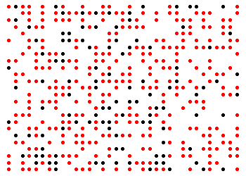
reft:TielFrankeSauerland2021 presented participants with displays like in Fig. 1, all of which consisted of 432 circles of which a variable number was red and the rest black. Participants then filled in whatever quantifying expression they found most appropriate to complete the sentence (with the exception of number terms, which they were told not to use):
We look here at the fifteen most frequently filled in quantifying expressions, together with the important but naturally less frequent options none and all. We take their their relative proportion of mentioning in the experiment as a (admittedly tentative) stand-in for the relative ease with which these expression may come to mind. We model the ease with which an expression comes to mind as a non-uniform utterance prior, instead of an utterance cost which would rather model an utterance’s production effort (see also Appendix Chapter 3 for more on this distinction).
var utterancePrior = Categorical(
  {ps: [0.02470356, 0.03013834, 0.10474308,
        0.03013834, 0.15217391, 0.02272727,
        0.06027668, 0.01432806, 0.04891304,
        0.01630435, 0.25691700, 0.01729249,
        0.01235178, 0.12252964, 0.03754941, 0.04891304],
   vs: ["about_half", "all", "almost_all", "a_lot",
        "few", "fewer_than_half", "half", "hardly_any",
        "many", "more_than_half", "most", "none",
        "several", "some", "the_majority", "very_few"]})
viz(utterancePrior)
The goal of the remainder of this section is to use these expressions (and their relative frequency) to account for imprecise focal ranges of these expressions. To keep things simple, we will not look at the actual production data from reft:TielFrankeSauerland2021 but rather rely on our own intuitions about plausibility of the model. The main points to demonstrate are: (i) how probabilistic pragmatic reasoning can cope with many utterances with their respective weights, and (ii) how to combine an RSA model with imprecise cardinality perception/representation.
A model for many quantifiers
We need to assume some semantics for our utterances. We do this by specifying lower and upper bounds for each quantifying expression.
var bounds = {about_half: [200,232],
              all: [432,total],
              almost_all: [410, total],
              a_lot: [120,total],
              few: [0,50],
              fewer_than_half: [0,216],
              half: [210,222],
              hardly_any: [0,10],
              many: [100,total],
              more_than_half: [216,total],
              most: [250,total],
              none: [0,0],
              several: [10,total],
              some: [20,total],
              the_majority: [250,total],
              very_few: [0,20]
             }
Exercise: Check this list to see if you find all the lower and upper bounds plausible (enough). Which ones would you like to change if any?
Here is a version of the scalar implicature model for a state space of 0, 1, …, 432 red circles and the above utterance set.
var total = 432

var statePrior = function() {
  return uniformDraw(_.range(total+1))
}

var uttFreq = [0.02470356, 0.03013834, 0.10474308,
               0.03013834, 0.15217391, 0.02272727,
               0.06027668, 0.01432806, 0.04891304,
               0.01630435, 0.25691700, 0.01729249,
               0.01235178, 0.12252964, 0.03754941, 0.04891304]

var utterances = ["about_half", "all", "almost_all", "a_lot",
                  "few", "fewer_than_half", "half", "hardly_any",
                  "many", "more_than_half", "most", "none",
                  "several", "some", "the_majority", "very_few"]

var utterancePrior = function() {
  categorical({ps: uttFreq, vs: utterances})
}

var bounds = {about_half: [200,232],
              all: [432,total],
              almost_all: [410, total],
              a_lot: [120,total],
              few: [0,50],
              fewer_than_half: [0,216],
              half: [210,222],
              hardly_any: [0,10],
              many: [100,total],
              more_than_half: [216,total],
              most: [250,total],
              none: [0,0],
              several: [10,total],
              some: [20,total],
              the_majority: [250,total],
              very_few: [0,20]
             }

// meaning function to interpret the utterances
var literalMeanings = function(utt, state) {
  var interval = bounds[utt]
  return (state >= interval[0] & state <= interval[1])
}

// literal listener
var literalListener = cache(function(utt) {
  return Infer({model: function(){
    var state = statePrior()
    condition(literalMeanings(utt,state))
    return state
  }})
})

// set speaker optimality
var alpha = 1

// pragmatic speaker
var speaker = cache(function(state) {
  return Infer({model: function(){
    // non-uniform utterance priors to model salience or ease-of-retrieval of
    // different expressions, rather than an utterance's cost / effort
    var utt = utterancePrior()
    factor(alpha * literalListener(utt).score(state))
    return utt
  }})
})

// pragmatic listener
var pragmaticListener = cache(function(utt) {
  return Infer({model: function(){
    var state = statePrior()
    observe(speaker(state),utt)
    return state
  }})
})
Exercises:
- Inspect the speaker’s choice of utterance for states 0, 432, 216 and 320 (the last one is instantiated in Fig. 1). Do you find these predictions intuitive? What could you change in the model to make them more to your liking?
- Use
viz.density()first and thenvizto visualize the pragmatic listener’s interpretation of some, few and many. In what way does this model (not) account for imprecise focal ranges?
Adding imprecision in cardinality perception/representation
When you look at a picture of 432 colored circles like in Fig. 1, it is rather unlikely that you immediately perceive with confidence that there are exactly 320 red circles. You might also not wish to count. Rather you might just activate a diffuse representation of the approximate number of red circles in this display. The Approximate Number Sense refp:Dehaene1997 is a formal theory that describes approximate cardinality representations in terms of a probabilistic penumbra, so to speak, around the true cardinality. We will take inspiration from this line of research and add a simple ANS module to our RSA pragmatic model.
The ANS approach assumes that the probability of perceiving or processing with number perceived_state when the true state is true_state is given by a normal distribution centered at true_state and a standard deviation that is a function of true_state as well. The motivation is that the probability of confusing a number n for n+10 is bigger the bigger n is itself. Usually, the standard deviation is assumed to be w times true_state, where w is the Weber fraction.
var total = 432

// possible states of the world
var statePrior = function() {
  return uniformDraw(_.range(total+1))
}

var weber_fraction = 0.2

// returns a state which is perceived when the true state is 'true_state'
var ANS = cache(function(true_state) {
  var true_state = Math.max(true_state, 0.01)
  Infer({method: "enumerate",
        model: function() {
          var perceived_state = uniformDraw(_.range(total+1))
          factor(Gaussian({mu: true_state,
                           sigma: weber_fraction * true_state}).score(perceived_state))
          return perceived_state
        }})
})

viz.density(ANS(432))
Exercises:
- Experiment with different activation curves for different numbers.
- Change the weber_fraction. What happens when it is increased? What happens when it is 0?
- Compare the curves for state 0 and state 432. Is this model appropriate for stimuli like in Fig. 1?
The ANS curves defined by the function above are not perfectly suited for displays like in Fig. 1 where there is a fixed total set size. The following symmetrized function takes care of the fact that, on the assumption that we know that there are 432 circles in total, mistaking a display with 430 red circles for one with 431 is equally like as mistaking one with 2 red circles with one with only 1.
var total = 432

// possible states of the world
var statePrior = function() {
  return uniformDraw(_.range(total+1))
}

var weber_fraction = 0.2

// returns a state which is perceived when the true state is 'true_state'
var ANS = cache(function(true_state) {
  var true_state = Math.max(true_state, 0.01)
  Infer({method: "enumerate",
        model: function() {
          var perceived_state = uniformDraw(_.range(total+1))
          factor(Gaussian({mu: true_state,
                           sigma: weber_fraction * true_state}).score(perceived_state))
          return perceived_state
        }})
})

var perceivedState = cache(function(true_state) {
  Infer({method: "enumerate",
        model: function() {
          var perceived_state = uniformDraw(_.range(total+1))
          factor(ANS(true_state).score(perceived_state))
          factor(ANS(total - true_state).score(total - perceived_state))
          return perceived_state
        }})
})
viz(perceivedState(2))
viz(perceivedState(430))
To add this module of approximate cardinality processing to the previous RSA model, the following code assumes that speakers have a probabilistic imprecise representation of the true cardinality but produce an utterance for the state which they perceive after possible perturbation with noise. (This is exactly like uncertainty was treated in the second model from Chapter 2).
var total = 432

var statePrior = function() {
  return uniformDraw(_.range(total+1))
}

var uttFreq = [0.02470356, 0.03013834, 0.10474308,
               0.03013834, 0.15217391, 0.02272727,
               0.06027668, 0.01432806, 0.04891304,
               0.01630435, 0.25691700, 0.01729249,
               0.01235178, 0.12252964, 0.03754941, 0.04891304]

var utterances = ["about_half", "all", "almost_all", "a_lot",
                  "few", "fewer_than_half", "half", "hardly_any",
                  "many", "more_than_half", "most", "none",
                  "several", "some", "the_majority", "very_few"]

var utterancePrior = function() {
  categorical({ps: uttFreq, vs: utterances})
}

var bounds = {about_half: [200,232],
              all: [432,total],
              almost_all: [410, total],
              a_lot: [120,total],
              few: [0,50],
              fewer_than_half: [0,216],
              half: [210,222],
              hardly_any: [0,10],
              many: [100,total],
              more_than_half: [216,total],
              most: [250,total],
              none: [0,0],
              several: [10,total],
              some: [20,total],
              the_majority: [250,total],
              very_few: [0,20]
             }

// meaning function to interpret the utterances
var literalMeanings = function(utt, state) {
  var interval = bounds[utt]
  return (state >= interval[0] & state <= interval[1])
}

// literal listener
var literalListener = cache(function(utt) {
  return Infer({model: function(){
    var state = statePrior()
    condition(literalMeanings(utt,state))
    return state
  }})
})

var weber_fraction = .4

// returns a state which is perceived when the true state is 'true_state'
var ANS = cache(function(true_state) {
  var true_state = Math.max(true_state, 0.01)
  Infer({method: "enumerate",
        model: function() {
          var perceived_state = uniformDraw(_.range(total+1))
          factor(Gaussian({mu: true_state,
                           sigma: weber_fraction * true_state}).score(perceived_state))
          return perceived_state
        }})
})

var perceivedState = cache(function(true_state) {
  Infer({method: "enumerate",
        model: function() {
          var perceived_state = uniformDraw(_.range(total+1))
          factor(ANS(true_state).score(perceived_state))
          factor(ANS(total - true_state).score(total - perceived_state))
          return perceived_state
        }})
})

// set speaker optimality
var alpha = 1

// pragmatic speaker
var speaker = cache(function(state) {
  return Infer({model: function(){
    var utt = utterancePrior()
    var perceived_state = sample(perceivedState(state))
    factor(alpha * literalListener(utt).score(perceived_state))
    return utt
  }})
})

// pragmatic listener
var pragmaticListener = cache(function(utt) {
  return Infer({model: function(){
    var state = statePrior()
    observe(speaker(state),utt)
    return state
  }})
})

viz(speaker(1))
viz.density(pragmaticListener("some"))
Exercises:
- Inspect the speaker’s choice of utterance for states 0, 432, 216 and 320 (the last one is instantiated in Fig. 1). Compare them to the choice of the speaker predicted by the previous model without ANS component. Do you find the new predictions more or less intuitive?
- Use
viz.density()andvizto visualize the pragmatic listener’s interpretation of some, few and many. In what way does this model (not) account for imprecise focal ranges?- What is the role of the Weber fraction for the pragmatic model? What happens if w goes up, for example?
Table of Contents